It has been quite a while since I have posted about astronomy and astrophotography. With yet another – holiday this time – weekend near the new Moon with cloudy skies, I thought it would be a good idea to write about the astronomy software I use for planning, general viewing, and imaging.

This first software post will focus on iOS applications. Future ones will cover the PC software I use. There are several iOS applications that I find very useful.

Darkness is a great app that gives you Sun and Moon rise/set times, Moon phase, and all the key twilight numbers. It is good to know astronomical twilight as that is when you can really start observing or imaging.

SkySafari is a very high-quality planetarium app for the iPad and iPhone / iPod. I use the standard version for basic object location but they also have enhanced versions that have features like telescope control. They also have Andriod versions.

Star Walk is very cool planetarium program that you can hold up to the sky and it will orient the image to show what you are looking at.

Emerald Sequoia has many interesting time-related apps. I find Observatory interesting for seeing where the Sun, Moon, and planets are on any day and time and Time which gives you exactly accurate time by contacting NTP servers.

As I said in my post at the end of August, a road trip was coming. There have been several more trips (one ongoing now) that have not allowed me the time to write a proper post.

When all this traveling is done, I will have a proper update.

It has been a busy August. We traveled to Upper Michigan to see my parents for a week. Getting there was an adventure, and not of the good kind.

There were thunderstorms south of Chicago so incoming flights were delayed. our flight was scheduled to leave at 6:50 pm and we boarded the plane at about 10:15pm. We sat for quite a while. They finally closed the doors, but then informed us that there was a mechanical issue with the cargo door. We then learned that that final delay pushed the crew beyond their maximum working hours under FAA regulations. So we all got off the plane.

The airline booked us into a hotel in Skokie. We finally got to the room (smoking, not non-smoking and it reaked of tobacco) at 1:15 am. We were up early and at the airport around 9am. Our flight finally left after noon. It was delayed 19 hours. It took longer to fly from Los Angeles to Marquette than is does to fly from Los Angeles to Mumbai.

The visit with my parents was good. Pleasant weather, many cousins around, good fun for all.

After catching up at work, I am off next week to take my older daughter to college. She is attending Gonzaga University in Spokane, Washington. We are planning a nice, scenic drive up US-395. Our first night will be in Alturas, California and the next day we make it to Spokane.

I had planned to return on a slightly more eastern route through Nevada. Thankfully, I was told about the Burning Man festival being held at Black Rock City through Labor Day weekend. Apparently, the traffic from the end of the festival turned a seven hour drive from Reno to Los Angeles into a 10 hour drive. I have now planned a different route.

On the return, I’ll leave Spokane mid-day and drive to Bend, Oregon. From Bend, I’ll head south on US 97, joining I-5 at Weed, California. Then a long day driving south on I-5 to Los Angeles.

Keeping up with my pace of an image every nine months or so, I finally got some data worth processing over the 4th of July weekend. I had high hopes for the weekend because with the 4th being on a Thursday, it was a four-day weekend almost exactly at the new Moon. Mother Nature intervened to reduce my imaging time, but I got enough data for an image.

My target was the Ring Nebula, or Messier 57. I wanted to image the extended, faint nebulosity surrounding this fairly bright planetary nebula. The night of July 4th I got 2 hours of hydrogen alpha (Ha) data in 12 10-minute sub exposures unbinned. On July 5th I got 35 minutes each of red, green, and blue in 7 (each) 5-minute sub exposures binned 2×2.

I had planned to get some luminance data and more Ha on the 6th, but it was cloudy at dusk. It was probably going to clear, but with astronomical twilight at 9:45 PM and M57 transiting at 12:45 AM, I decided to take my calibration frames and call it a night. Perhaps I’ll get more data later this summer, but I decided to process what I had.

My initial approach was to create a synthetic luminance image from the RGB data, combine that with the Ha data for a final luminance, and then add color from the RGB. Note that my RGB data is binned 2×2, so I don’t have the full definition of my camera for anything but the Ha data. My second approach was to also add Ha to the red channel. That produced the best result.

Overall, the image is noisy because there is limited data and everything but the Ha was taken at 2×2. I was somewhat aggressive with ACDNR noise reduction. I admit up front this is far from a perfect image. But it is what I could get with the data I have.

Here is the final image

M57 HaRGB Version 2

Here is my initial pass at processing

M57 HaRGB Version 1

What follows is a more detailed description of the processing steps.

Continue reading →

In my post on darks and biases below, I combined a small and a large number of frames to create master frames and see how much difference could be seen in the master frames. I have now repeated the experiment in PixInsight and have some more quantitative result.

The overall result is the same: The difference in the bias frames is quite noticeable, the difference in the darks is hard to discern, and any difference in the final calibrated light frames is hard to see at all.

On further analysis, these results make sense. A bias is the base level readout from the camera and is subject to read noise. The base level readout — the bias — is a very low signal. The average bias pixel value is about 0.00162 on a 0-1 scale or about 106 on a 16 bit basis with maximum values of 0.00678 (0-1) or 444 (16-bit). With a low signal, the read noise would be more visible and an the reduction in noise from the increase in integrated frames is more visible.

With darks, we are capturing both the bias and the dark noise. The dark noise is greater than the bias (otherwise we would not need to take darks). The dark has an average value of 0.00174 / 114 (same units as above) which is about 7% higher than the bias, but has a maximum value of 0.859 / 56,300. With this greater signal and larger variance, it is harder to see the difference from a larger number of frames than with the bias. The dark noise itself is noise, and a larger number of frames gives us a better measure of that noise. That increase in quality I do not think is visible. It should contribute to a better final image. In the images below, I have stretched the dark and bias frames identically, so there is some difference visible between the low and high number of integrated frames.

Finally, with the light frames, the signal is much greater than the dark with an average value of 1.5 greater after calibration and 2.4 times greater before calibration. In addition, my frames are dithered so that the camera based noise (like dark noise and bias) are spread out among the subframes and minimized during image integration through data rejection.

First, let’s look at the biases. I combined 48 and 148 frames to make two different master bias frames. The frames were averaged without normalization or weighting. I used a Winsorized Sigma Clip with a high and low sigma factor of 3.0. The combination yielded the following noise evaluation results:

Integration of 48 images:
Gaussian noise estimates: s = 1.677e-005
Reference SNR increments: Ds0 = 1.1788
Average SNR increments: Ds = 1.1784

Integration of 148 images:
Gaussian noise estimates: s = 9.742e-006
Reference SNR increments: Ds0 = 1.4379
Average SNR increments: Ds = 1.4362

To put the numbers in perspective, the overall noise is 42% lower and the SNR is 22% higher, assuming I am interpreting the numbers correctly.

Master bias integrating 48 frames:

Bias from 48 frames

Master bias integrating 148 frames:

Bias from 148 frames

I discovered a very nice feature in PixInsight while performing this experiment. In the original test, I used 44 and 80 frames to create the master darks. PixInsight will report how many low and high pixels are rejected for each frame being integrated. When I looked at the log, I saw that the first frame had a very high number of pixels being rejected:

1 : 1150170 35.777% ( 516 + 1149654 = 0.016% + 35.761%)

At the time I started taking the flats, the “simple cooler” command I used in CCDCommander did not wait for the camera to cool fully before taking the darks. It got down to temperature fairly quickly, but apparently not quickly enough. The images below exclude that dark frame from the masters.

The master dark integration settings were identical to the ones used for the biases. Here are the statistics from the dark integration:

Integration of 43 images:
Gaussian noise estimates: s = 2.499e-005
Reference SNR increments: Ds0 = 2.8991
Average SNR increments: Ds = 2.6725

Integration of 79 images:
Gaussian noise estimates: s = 2.064e-005
Reference SNR increments: Ds0 = 3.2427
Average SNR increments: Ds = 3.2073

The noise decreases by 17% and the SNR increases by 20%, again if I am interpreting the statistics correctly. It is somewhat ironic that the signal in this case is noise. But it is that noise we are trying measure by taking darks.

Master dark integrating 43 frames:

Dark from 43 frames

Master dark integrating 80 frames:

Dark from 79 frames

Of course, the whole reason for calibration is to create a better light image. I processed my light frames from NGC 925 taken in early December using the two different sets of masters. Different masters were used to calibrate both lights and flats. I used dark optimization during calibration. All lights were aligned to the same frame using nearest neighbor resampling. I used an average combine, multiplicative output normalization, scale+zero offset normalization for rejection, and Winsorized sigma clipping with a clip setting of 2.2 on both high and low pixels.

Integration of 36 images using 48 bias and 43 darks:
Gaussian noise estimates: s = 4.955e-005
Reference SNR increments: Ds0 = 3.7736
Average SNR increments: Ds = 3.6726

Integration of 36 images using 148 bias and 79 darks:
Gaussian noise estimates: s = 4.947e-005
Reference SNR increments: Ds0 = 3.7751
Average SNR increments: Ds = 3.6744

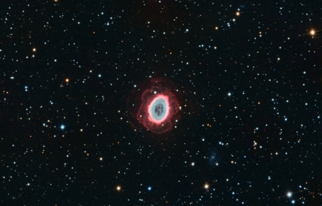
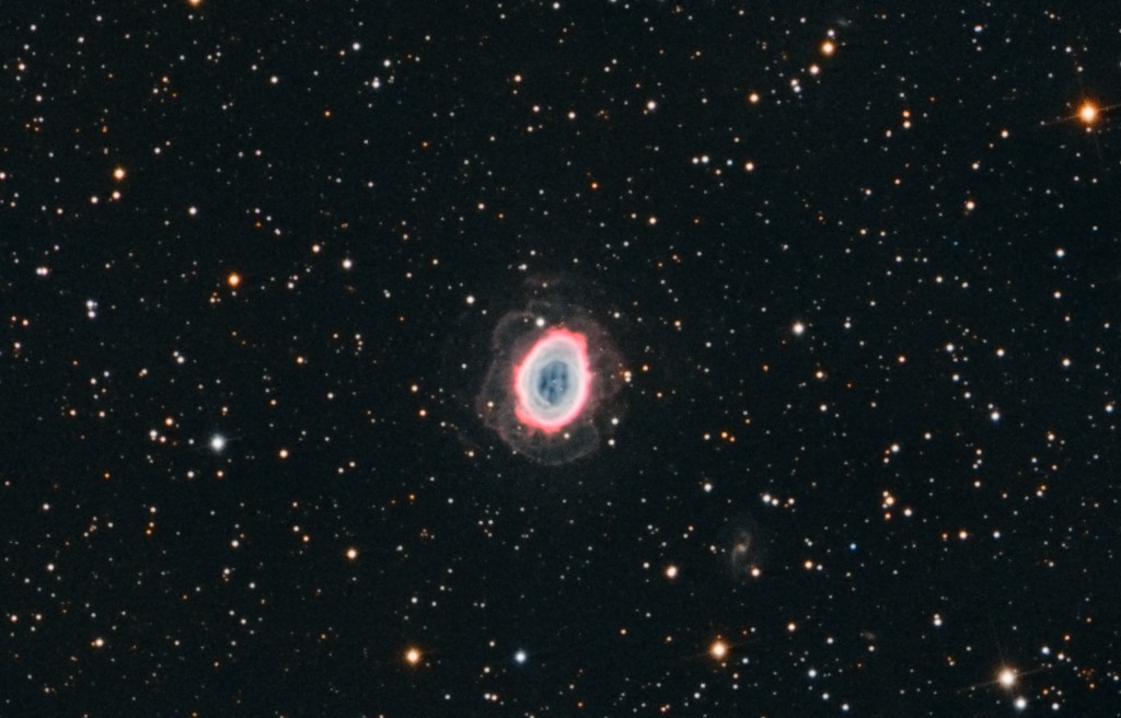
This is a 0.16% decrease in noise and a 0.05% increase in SNR. Not a huge statistical improvement and, to my eye, not visible in the final image. The two lights below are stretched to the noise floor or beyond and it is difficult to say that one is better than the other. Both are stretched identically. The image artifact in the upper right showed up on my second night of data gathering and I suspect it is from frost in the camera.

NGC 925 processed with bias master 48 and dark master 43:

NGC 925 calibrated with a smaller number of Bias and Darks

NGC 925 processed with bias master 148 and dark master 79:

NGC 925 calibrated with a large number of Bias and Darks

There is no great illuminating conclusion to this analysis. Certainly, take all the darks and biases you can. There is a real improvement in the bias quality and they don’t take a lot of time. I am going to try to get another 100 darks to see if I get any improvement, but I feel once you are in the 40s the increase in quality is small. I may do this experiment with my color frames, which are binned 2×2 and have much lower signal than the luminance I used here.

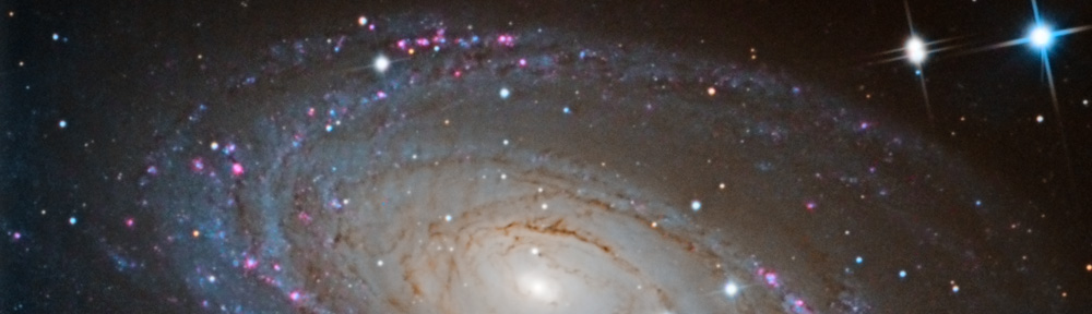
Finally, here is the high-number calibrated NGC 925 stretched to look decent, just so everyone knows it is a nice image. Check out the fully processed LRGB NGC 925 in the gallery, too.

NGC 925 with a normal stretch

Common practice and solid math tell us that more dark and bias calibration frames in your master, the better. More is better, but how many more? To find out I have created as set of 1×1 binned test images. The darks are from 44 and 80 images and the biases are with 48 and 148 frames. Interestingly, I cannot see any difference between the two darks. They seem identical. The biases, on the other hand, are very different, with the bias produced using 148 frames having an obviously lower amount of noise.

It looks like, as expected, more frames are better. But I think I need to get another 100 or so darks to see if I have a similar difference to the bias frames. 44 to 88 dark frames didn’t seem to make a difference. Will having 150 dark frames make a difference?

The frame combination was done in CCDStack using a sigma clip mean combine and a sigma factor of 3.0. I think I need to try a version using PixInsight. Although I do my data reduction in CCDStack because PixInsight does not have bloom removal, and CCDStack’s bloom removal works very well.

The two bias frames, 148 frame version on top

148 frame bias

48 frame bias

The two dark frames, 80 frame version on top

80 frame dark

44 frame dark

AIC 2012 has wrapped up. A very fine conference this year with a lot of great content and many good times talking about imaging and astronomy. The day finished with great door prizes, which was fun even if I didn’t win one. There were also two excellent presentations.

John Smith presented How get The Most from your Imaging System. It is all about noise. As little as possible, that is. Noise comes from read noise, sky glow noise, dark noise, and signal noise. Measure your noise in electrons (convert backward from your camera’s gain and an image’s ADU). Noise is the square root of the electron signal. For most imaging, you want to drown the read noise with sky glow noise. CCDWare has a calculator for subexposure length to find the optimal length.

Dithering — moving the camera by a couple of pixels between subexposures — is critical. John recommends a fixed rather than a random dither pattern to ensure no two exposures are in the same place. With good dithering, John believes one might be able to image without using darks!

On your set-up, automation produces more consistent results because your set-up is stable. Make sure your cables are well managed. John likes to put all power distribution and communication on the scope, with only 12 volt and a single USB cable coming down off of the mount. Be creative in how you attach items to the mount. Always use professional grade hubs and serial to USB adapters.

The final presentation was from Alan Erickson, a lead engineer on Photoshop, discussing Image Processing. He presented many tips and tricks with Photoshop which are too detailed to present here. I’ll be looking forward to getting a copy of his presentation. Again I saw how deep Photoshop is as a tool.

Many thanks to Ken Crawford and the whole team that put together yet another amazing conference!

AIC 2012 day two has been excellent. After a fine breakfast, we started with the Hubble Award lecture from honoree Adam Block. He demonstrated some of the techniques that make him such a renowned imager and the excellent teaching style that makes his out reach and tutorials so effective. Alistair Symon followed with a good presentation on making wide field mosaics using Photoshop and Registar.

After the break, Travis Rector spoke on Presentation Quality Image Processing. He had some very good lines in his talk including “Astrophotos are like your children, you love them because they are yours not because they are pretty.” Working for the observatories, he is careful not to use any aggressive processing on the image, and he still gets emails with people seeing hidden aliens in image processing artifacts.

He hit the key points in the ongoing discussion of “what does it really look like?”. Or as he said, it doesn’t look like the picture because:

• surface brightness is constant, if you are closer to the object you still couldn’t see it
• People can’t see color in faint light
• Our eyes have poor sensitivity to red light
• Processing compresses the dynamic range does not match direct perception
• Filters and wavelength go beyond visual

So asking what it looks like is a meaningless question. Travis tries to translate what a telescope can see into what we can appreciate. That is his art and he does it very well. Everything he does in processing is done with curves and levels, and he follows some simple rules:

• Know your object – do research and plan what data to capture
• Take educated risks – try what others haven’t
• Crop and rotate to show what you want the viewer to see
• Use color well
• Surface brightness is your friend as an amateur – big scope, you get more small dim objects, smaller scope higher f ratio better on larger objects

Check out the paper Image processing techniques for the creation of presentation quality astronomical images. Available at Arvix.org/abs/Astro-ph/0412138/. (I’ll fix the URLs later)

After lunch we had an excellent talk from UC’s Geoff Marcy on the Hunt for Exoplanets. Then Astronomy magazine’s David Eicher spoke on the Future of Amateur Astrophotography.

The Spotlight presentations were very good. Tom Field presented Simple Spectroscopy. There is a range of options from $200 to $2,000+ for doing spectra, and it is real science. A very enthusiastic presentation. He told a great story about how a strange emission line was seen in a spectra of the sun taken during an eclipse. It did not match any known element. So the unknown element was named Helium for the sun, Helios. Years later, the spectra was seen from a gas coming from decaying uranium. That gas was helium, now really found.

Jerry Bonnell presented on Planetary Nebula on behalf of Don Goldman. Excellent theoretical background was provided. Apparently the hourglass shape of the nebulae comes from the fast moving later stellar pushed above and below the rotation axis by slower stellar winds that primarily go on the rotation axis. All of this is occurring as the star goes through its giant phase at the end of its life.

Sal , a young astrophotographer from Florida, presented on Astrophotography Under Light Polluted Skies. He presented an excellent set of Photoshop centric approaches for producing good images. This included Jay Gabany’s layered contrast stretching approach that, once I get Sal’s presentation I might actually understand how it is done. Sal recommends RGB at 1×1 and same duration as Luminance, combining the RGB with Luminance for a master luminance frame. This FITS my experience when imaging in the city. His paint bucket on background smoothing seems like adding data to me, so I’d avoid that.

Excellent times with the vendors. Altogether a good day!

AIC 2012 has begun! Day one has been filled with some excellent sessions. The exhibitor hall is open and there will be a two-hour opening later this evening.

My first session today was Ron Wodaski’s introduction to PixInsight. He covered many of the basics (that’s a lot) and gave some glimpses of the advanced features in the platform. Even an experience PixInsight user like me found it a useful and informative presentation. I am looking forward to seeing the full deck with all the details Ron promised.

I then attended Tim Puckett’s presentation on supernovae searching. He has built some amazing telescopes and quite a robust process and team for finding supernovae. When it is clear, his team will image 2,000 galaxies to find potential supernova. I learned that fit order 3 or 4 is required in PinPoint for astrometric reporting, and how to access the reference magnitude function in Maxim DL.

After lunch, there was a great presentation by Steve Brady, co-developer of the great focusing program, FocusMax. FocusMax uses the idea that there is linear relationship of the half flux diameter or HFD to focus that can be used to quickly and accurately focus a telescope using a CCD. HFD is the circle that evenly splits the flux or total ADU of a star regardless of focus. It is expressed in pixels. Max flux for a system is best calculated by plotting max pixel and max flux vs. time and picking a max flux value below where the curve flattens out. Focus convergence was clearly shown to be the best way to get to focus, even though it takes longer than the default of 5 exposures.

There was a very interesting discussion on precision vs. accuracy in FocusMax, and the key point is the size of the critical focus zone. More reading will be needed on that later. Focus is driven by the Vcurve, which is a hyperbola. Fit of measurements in creating a Vcurve are fit to the hyperbola, not to a linear fit of each side of the v. One should pick the point just above where the Vcurve moves away from the line as the near focus HFD, with the start HFD being about five units higher. Get at least 12 Vcurves for best results.

A major new release is coming sometime in the relatively near future. For now, the beta version is quite stable and is the one to use.

Finally, there was a great presentation from Ken Crawford on using masks in Photoshop CS5. I think I understand alpha channels now — they are containers for masks. He will have a video tutorial for all AIC attendees.

I took this image of NGC 7814, a spiral galaxy in Pegasus, last November but only am getting around to posting it now. I am afraid that the color is a little weak in the blue, but I’m not up to going back to the drawing board on this one. Click on the image for a full sized version and more information in the gallery.